
What I'm Learning: EKF SLAM & ORB SLAM2
I miss blogging, and I thought it would keep me focused to publish a short post about what I’m learning, or what projects I’m working on, each week.
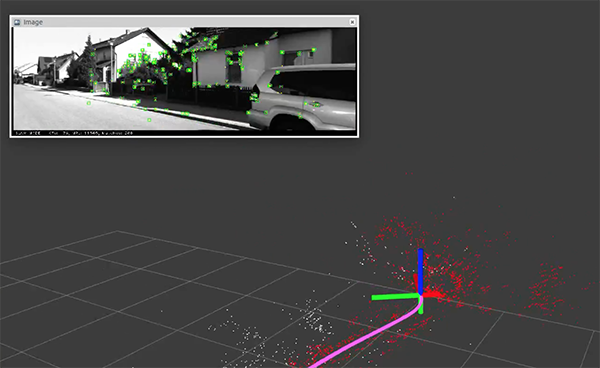
Pictured, ORB SLAM2 in action, screenshotted from Louis Zhang’s ROS demo
Over the last few weeks I’ve been studying EKF SLAM and ORB SLAM2 (paper). For the uninitiated, EKF stands for Extended Kalman Filter, a generalization of Kalman Filters (KF). KFs are realization of the Bayesian Filter paradigm, and EKFs are an enhancement of KFs that deal better with non-linear circumstances. Bayesian Filters are used heavily in autonomous vehicle platforms (or more generally, robotics), particularly to bring together multiple sensors sources (sensor fusion), to generate or maintain maps of an area (mapping), or to identify where a robot is (localization).
EKF SLAM (Cyrill Stachniss lecture) is the specific application of an EKF to the SLAM problem, where SLAM stands for Simultaneous Localization And Mapping. SLAM is the task of creating a map of the robot’s environment in real time, while also tracking where the robot is in that environment. To understand SLAM, think about when you enter a new room. Your visual cortex conveniently builds a map of the new room for you (a sense of where everything is), and as you walk around the room, your visual cortex keeps track of where you are within that map. Without thinking about it, you learn the shape of your new surroundings and know where you are in it. The brain is amazing, which you learn when you try to replicate this feat for self-driving cars = SLAM is very difficult.
With EKF SLAM, I’ve reached a point where I understand all the steps of the algorithm (with known data association) at each level, and I’m thinking now of building up a prototype implementation in C++ as an exercise. I haven’t dove into EKF SLAM where data association is inferred, but will do so soon. EKF SLAM is not performant in real world circumstances for most robots or autonomous vehicles, but it’s a sort of MVP of SLAM algorithms, so understanding it gives you a good grip on the foundations of the SLAM process.
For ORB SLAM2, I’ve been reviewing the top level process flow, and also digging into definitions. It’s surprisingly hard at times to find root definitions without diving into a chain of papers. For example, while studying the paper on my phone in the car, I ran across the term BA, in the title of the algorithm, ORB. What the heck do these mean? Figuring out with Google what BA stands for (bundle adjustment) or ORB (Oriented FAST and Rotated BRIEF) was actually a bit of work. There’s a need for a autonomous vehicles glossary, for anyone who wants to make a name for themselves.
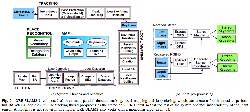
ORB SLAM2, unlike EKF SLAM, is real production algorithm that can operate in large environments under real conditions, for example, here’s a video of ORB SLAM in action using the KITTI dataset. And here’s video of ORB SLAM2 working in indoor environments. This high level process diagram for ORB SLAM2, taken from the original paper, really highlights the complexity:
∆ between EKF SLAM and ORB SLAM2
There are some key differences between EKF SLAM and ORB SLAM2 that illustrate the difference between a very elegantly stated but usually impractical algorithm - EKF SLAM with known data correspondence - and a less mathematically simple algorithm that can actually succeed in production environments - ORB SLAM2:
- Data correspondence: EKF SLAM assumes that, when given measurement data for known landmarks, it knows which measurements correspond to which landmark. By contrast, a large part of ORB SLAM2 is a feature identification and matching pipeline, which finds ORB features (ORB is a patch descriptor) in each keyframe, and identifies any likely matches in other key frames based on the ORB vector. In practice, production SLAM, mapping, or localization algorithms need some kind of pipeline providing features, and a means to match them up across frames.
- Global vs local belief updates: EKF SLAM essentially updates it’s beliefs for all landmarks at all times (this is not exactly true), even if a landmark is far far away from the robot’s location. It would be analogous to you updating your map of London when you come upon a detour in Los Angeles: impractical and unnecessary. ORB SLAM2 restricts updates to a local map, unless specific measurements suggest that a global update is needed, which is a lot more efficient if you can make it work.
- It was not immediately obvious (to me) that when one landmark’s belief is updated in EKF SLAM, all are. It occurs because, while EKF SLAM only directly updates the mean location for one landmark measurement (say landmark $j$) at a time, the covariance matrix $\Sigma_t$ will eventually correlate all the landmarks with one another, and thus updates to $\bar{\Sigma}^j_t$ will not be isolated to rows pertaining only to landmark $j$.
- Loop closure: Imagine driving around the block. A robot can do this while building a map, but will often find that when it finishes driving around the block that, in its map, the start location is offset from the end location (which are the same) by maybe 10 meters. At this point the mapping algorithm needs to recognize that these locations are the same and adjust the map to reflect that. And go back and adjust all the flaws in the map that led to the start and end point not aligning. This is referred to as
loop closure. EKF SLAM handles this via the naive assumption that data correspondence is known, and by constantly updating all landmarks. However, this proves to be computationally intractable, and not realistic, and ORB SLAM2 implements a whole system for handling this circumstance efficiently.- Example of, what appears to be, loop closure in EKF SLAM @ 0:35.
- Example of loop closure in ORB SLAM2 @ 0:46.
That’s enough for now, back to the grindstone.