Simultaneous Localization and Mapping Cheatsheet

Learning SLAM has sent me far and wide across the internet to track down key terms and resources, so to solve that problem for others, I’m maintaining a growing cheatsheet of SLAM resources and terms here as a quick reference.

This is a work in progress, so suggest new items or revisions, or let me know what you think by emailing me, or leave a comment below.

Resources:

• Cyril Stachniss’ 22 lectures @ Uni Freiburg on SLAM at Uni Freiburg (2013/14) on YouTube
  • Syllabus, slides, other links for the course
• Gil Levi provides a gentle introduction to feature-detector-descriptors
• Github user kanster aka robotics researcher Kanzhi Wu’s list of SLAM resources. Mr. Wu’s resources have been immensely helpful to me at times, I highly recommend them.
• Probabilistic Robotics by Thrun, Burgard, and Fox is a fantastic book and is the foundation for Cyril Stachniss’ lecturs.
  • Amazon
  • Preprint

Selected papers

These papers concern cutting edge techniques in SLAM, or support those techniques.

• ORB SLAM and ORB SLAM2:
  • ORB SLAM2 codebase
  • Monocular ORB SLAM paper via Raúl Mur-Artal, J. M. M. Montiel and Juan D. Tardós. ORB-SLAM: A Versatile and Accurate Monocular SLAM System.
  • Stereo & RGB-D ORB SLAM2 paper via Raúl Mur-Artal and Juan D. Tardós. ORB-SLAM2: an Open-Source SLAM System for Monocular, Stereo and RGB-D Cameras.
  • DBoW2 technique for place recognition via Dorian Gálvez-López and Juan D. Tardós. Bags of Binary Words for Fast Place Recognition in Image Sequences.

Glossary:

• AKAZE: Accelerated-KAZE is a multiscale feature-detector-descriptor algorithm that innovates on KAZE using a technique called Fast Explicit Diffusion. The details of AKAZE originated in the 2013 paper Fast Explicit Diffusion for Accelerated Features in Nonlinear Scale Spaces and AKAZE features are implemented in OpenCV.
• Bayes Filter (aka Recursive Bayesian Estimation): a recursive predictive modeling paradigm that works particularly well for online applications like SLAM or sensor fusion. Kalman filters and particle filters are two popular examples of Bayes filters.

• $bel(x_t)$ (Bayes filters): the belief at time $t$, this is the updated state after fusing the prediction at time $t$ with the measurement at time $t$:

  $$bel(x_t) := p(x_t \ | \ z_{1:t}, u_{1:t}) = \eta \underbrace{p(z_t \ | \ x_t)}_{\text{measurement model}} \underbrace{\overline{bel}(x_t)}_{\text{recursion}}$$

  where $\eta$ is the normalizing constant that normally arises from Bayes Rule, in this case:

  $$\eta = p(z_t \ | \ z_{1:t-1}, u_{1:t})^{-1}$$

• $\overline{bel}(x_t)$ (Bayes filters): sometimes called prediction at time $t$, I sometimes call it belief after prediction, this is the belief after predicting the next state but before incorporating the new measurement:

  $$\overline{bel}(x_t) := p(x_t \ | \ z_{1:t-1}, u_{1:t}) = \int_{x_{t-1}} \underbrace{p(x_t \ | \ x_{t-1}, u_t)}_\text{motion model} \ \underbrace{bel(x_{t-1})}_\text{recursion} \ dx_{t-1}$$
• Bundle Adjustment (BA): the process of taking the adjusting the location of 3d features observed, adjusting camera pose, and adjusting camera calibration parameters to optimize for maximum likelihood. Mathematically this essentially involves minimizing the reprojection error between the image locations of observed and predicted image points. BA is broadly used, and thus often customized to the circumstances. For example, you might find that in one application only some camera poses are allowed to vary, and in another application, pose constraints between cameras are stronger.
• Camera Pose: the orientation and location of a camera.
• Disparity: the difference in a feature’s location in two images. In a stereo system, this would typically refer to the difference in x-coordinate of a feature’s location in stereo rectified pair of images. In a monocular system, this might refer to the change in position of a feature after the camera’s pose has changed.
• Extended Kalman Filter (EKF): a Bayes Filter which is an extension of the Kalman Filter approach. Extended Kalman Filters cope better with non-linear motion and observation models than do Kalman Filters. It does this by linearizing these motion models at the relevant points using the function Jacobians. To quote Cyril Stachniss “[EKF] just does everything to fix KF for non-linear models based on ‘stupid’ [air quotes] linearization” :) .
• Feature Detector: any algorithm that processes image or point cloud data and identifies distinctive features in the image or point cloud. Usually you want your feature detector to detect the similar (or the same) features from different points of view, at different scales, and under different environmental conditions, so that the features provided to your SLAM algorithm are mostly invariant to these factors. Detected features usually end up as keypoints in the image and map points in the map.
• Feature Descriptor (or Patch Descriptor): any algorithm that, given a feature location in image or point cloud data, generates a representation of the feature. These descriptors are then typically used to match covisible keypoints across frames, and then with triangulation, create corresponding map points and estimate their location. As with detection, usually you want your feature detector to detect the similar (or the same) features from different points of view, at different scales, and under different environmental conditions, so that the feature matching is consistent under different conditions.
• Feature-Detector-Descriptor: an algorithm that both detects and describes features. Some examples are HOG, ORB, BRIEF, SIFT, SURF, KAZE and AKAZE. A series of posts by Gil Levi provides a gentle introduction to feature-detector-descriptors.

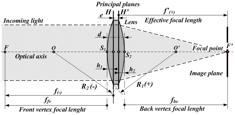
• Focal length: the distance $f$ for a given camera system at which parallel rays of light meet at a focus in the image plane. In an ideal pinhole camera model, $f = f_x = f_y$, but in practice it is often true that camera calibration shows $f_x \neq f_y$. See below $f_{bv}$, the distance between the focal point $F^\prime$ and the last optical surface $S_2$:

  

• Gauge Freedom: freedom in the choice of coordinate system. For example, by convention, when starting up a SLAM algorithm, the first keyframe is typically assumed to be located at the origin, with no rotation, but you are free to choose otherwise. Gauge freedom and the fix for it, [gauge fixing, is a big thing in physics](https://en.wikipedia.org/wiki/Gauge_fixing, but not a big worry in robotics, so far as I can tell.

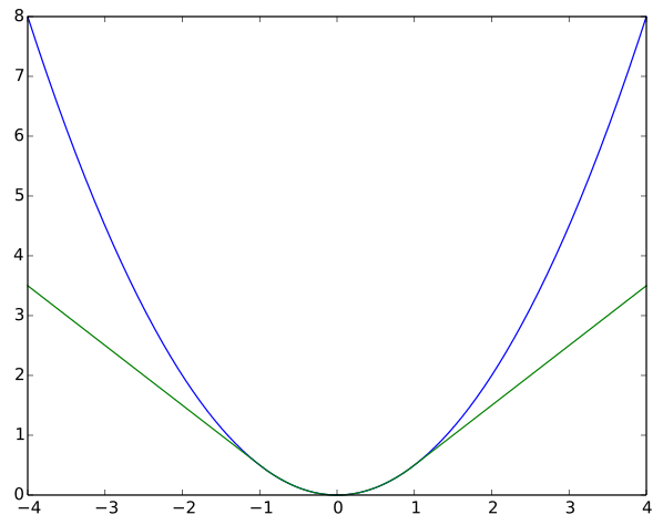
• Huber loss: a loss function that places less weight on outliers. It is essentially a mix of the squared loss and absolute loss, configured to be once differentiable. Definition of the Huber loss function with parameter $\delta$, $L_\delta(a)$:

  $$L_\delta(a) = \begin{cases} \frac{1}{2}a^2 & |a| \leq \delta \\ \delta(|a| - \frac{1}{2} \delta) & |a| > \delta \end{cases}$$

  Huber loss function with $\delta = 1$ (green) vs 1/2 the squared loss function (blue):

  

• KAZE: a multiscale feature-detector-descriptor algorithm which aims to address noise problems but retain object boundaries. In Japanese KAZE means wind, a reference to flow ruled by non-linear processes, and is an indirect tribute to Taizo Iijima, the father of scale space analysis. KAZE originated in the 2012 paper KAZE Features and are implemented in Open CV.
• Iterative Closest Point (ICP): an algorithm for matching up similar point clouds. The tl;dr version of this algorithm is (1) find the closest matching points between the two clouds, (2) estimate the transformation which gives the best match, (3) transform the clouds with this transformation, (4) iterate until you reach a satisfactory threshold (or the solution fails to converge.) Like bundle adjustment, ICP tends to be implemented differently according to the circumstances of the application.
• Kalman Filter (KF): a specific class of Bayes filters that assumes that the motion and observation models are linear with Gaussian noise. In this case, it can be proven to be the optimal solution. If the underpinning reality is somewhat non-linear with not-very-Gaussian, the filter performance will tend to suffer accordingly. Kalman filters and their generalizations such as Extended Kalman Filters and Unscented Kalman Filters are heavily used in robotics for numerous tasks, from vehicle tracking, to sensor fusion, to SLAM.
• Keyframe: a frame that contributes information to the SLAM task. At 15 or 30 frames-per-second, it’s problematic to use all frames to accomplish SLAM, so typically SLAM algorithms select only a percentage of frames to contribute, called keyframes. Keyframe selection procedures can make or break some algorithms.
• Lambertian Reflectance: the ideal for reflection of light by matte surfaces. A surface with Lambertian reflectance has the same brightness regardless of the observer’s point of view. Feature-detector-descriptors tend to perform better on Lambertian surfaces, in that they are more likely to correctly match the feature when seen from different angles.
• Localization: identifying the robots position with respect to a map or coordinate system.
• Loop Closure: identifying when the robot visits a location it has been to before, updating the map to reflect that the match between the current location and the previous location, and reconfiguring the map to correct any accumulated drift the loop closure reveals.
• Map Reuse: when a map, usually built with SLAM, is later reused for localization, typically localization only.
• Mapping: building a map of the environment with the robot’s sensor data.
• Measurement Update (or Observation Step): the second of the two steps to recursively update a Bayes filter, the measurement update follows the prediction update. The measurement step takes a belief description (often a mean and covariance matrix, $(\bar{\mu}_t, \bar{\Sigma}_t)$) from the prediction update, a measurement, and noise characteristics of the measurement model and updates the belief. Alternatively, just think of it as the calculation of $ bel(x_t) $ from $ z_t $ and $ \overline{bel}(x_t) $.
• Metric Scale: when the relationship between the scale of the map’s coordinate system and the real world is known, we say the map has metric scale. Example: if you knew that 1.0 units in the map scale translated to 3.3 feet in the real world, you map has metric scale.
• Minimum Spanning Tree: a spanning tree for a edge-weighted graph that has the minimum total edge-weight of all such graphs. A spanning tree is a tree that connects all vertices in a connected graph.
• Motion Model: a state transition model that assigns a probability to the robot’s new state $x_t$ based on the previous state $x_{t-1}$ and the previous controls $u_t$. The model is the probability $p(x_t \mid u_t, x_{t-1})$. It is used in the prediction update in a Bayes filter. Usually this model is derived from (1) a set of motion equations and (2) a description of the process noise.
• Observation Model (or measurement model): a state transition model that assigns a probability to a measurement $z_t$ based on the current state $x_t$. The model is the probablity $p(z_t \mid x_t)$. It is used in the measurement update of a Bayes filter. Usually this model is backed by (1) a set of equations describing how the state space projects onto measurement space and (2) a description of the measurement noise.

• ORB: stands for Oriented FAST and BRIEF. This is a computationally efficient feature-detector-descriptor that is approximately invariant under rotation and scaling, and resilient to camera auto-gain, auto-exposure, and illumination changes. Here’s an example of ORB feature matching showing a Valentine’s card (left) feature matching with a smaller version, right, drawn via Hian-Kun Tenn (YouTube):

  

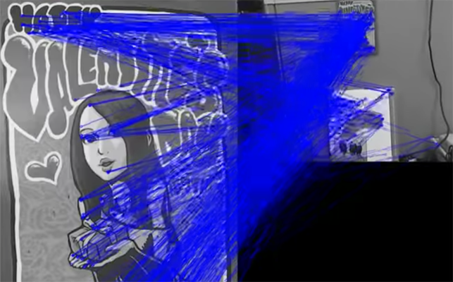
  ORB features were originally described in E. Rublee, V. Rabaud, K. Konolige, and G. Bradski, “ORB: an efficient alternative to SIFT or SURF,” in IEEE International Conference on Computer Vision (ICCV), Barcelona, Spain, November 2011, pp. 2564–2571. They are implemented in OpenCV.

• Prediction Update (or Prediction Step): the first of two steps to recursively update a Bayes filter. When the filter receives a new measurement, it first executes a prediction update, guessing where the state space should land given the current information, including recent controls. It then incorporates the new information provided by the measurement in the measurement update. The prediction step takes belief from timestep $t-1$ (often a mean and covariance matrix, $(\mu_{t-1}, \Sigma_{t-1})$), and updates the belief according to the motion model. Alternatively, just think of it as the calculation of $ \overline{bel}(x_t) $ from $ u_t $ and $ bel(x_{t-1}) $.

• Principal Point: the principal point is the point on the image plane onto which the perspective center is projected. As well, it is the point from which the focal length is measured (Source: PCI Geomatics). In the context of computer vision, it will be the image coordinates $(c_x, c_y)$ of the principal point $\mathbf{P}$ in the diagram (Source: Princeton COS 429: Camera Geometry) below:

  

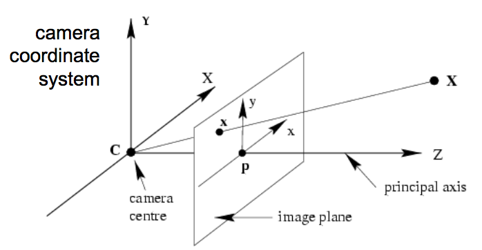
  So, in the case of 640x480 image, if the principal point were the dead center of the image, then $(c_x, c_y) = (319.5, 439.5)$.

• Projection: refers to projecting the elements of a 3D scene onto a camera plane, based on the known camera pose and optics. For instance, for an image plane at the origin, with focal length $(f_x, f_y)$ and principal point $(c_x, c_y), the projection function is:

  $$\pi\left( \begin{bmatrix} X \\ Y \\ Z \end{bmatrix} \right) = \begin{bmatrix} f_x \frac{X}{Z} + c_x \\ f_y \frac{Y}{Z} + c_y \end{bmatrix}$$
• SLAM: Simultaneous Localization and Mapping, a process by which a robot, or robots, simultaneously (1) build a map of the environment and (2) track their position in with respect to that map. Typically this is done in real time to assist the robot in understanding, interacting with, or navigating the environment.

To be added:

• Image Registration:
• RGB-D:
• Reprojection Error:
• Rolling Shutter:
• SIFT:
• Photometric Error:
• Pose Graph:
• Pose:
• SURF:
• Scene Point (or Map Point or Mappoint):
• Similarity Transformation:
• Spanning Tree:
• Stereo Baseline:
• Stereo Disparity:
• Triangulation:
• Unscented Kalman Filter (UKF):
• Up To Scale:
• BRISK
• Affine Transformation:
• SO(3):
• Lie Algebra:
• Visual Odometry:
• Relocalization:
• Particle Filter:
• Point cloud registration:
• ORB SLAM:
• ORB SLAM2:
• EKF SLAM:
• Graph-Based SLAM:
• Sensor Fusion:
• Bag of Words Place Recognition:
• Markov Assumption: