Tuning Extended Kalman Filter Process Noise with Discriminant Training

TL;DR: Using Discriminative Training of Kalman Filters (2005) to your tune filter’s process noise.

I recently was asked about how you tune the noise covariance matrices for (Extended) Kalman Filters. It was a pointed question, where I felt obliged to have an answer, and while I had a good answer for the measurement noise $R$, I could only remember iteratively hand tuning $Q$ based on some educated guesses and perceived performance. I assumed there was a better answer, and I was embarrassed I didn’t have it, so I set out to find it.

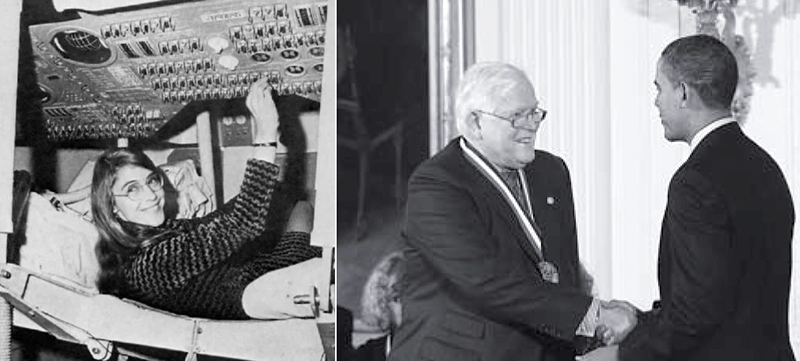
Right: Rudolf Kalman, inventor of the Kalman Filter, receives the National Medal of Science from President Obama. Left: Margaret Hamilton, one of the leading minds who developed the Apollo on-board flight software, sits in the Apollo module. The navigation system interface is above her head, below the circular attitude indicator, running Kalman’s filter.

As it turns out, tuning $Q$ is hard, it is typically done by hand, there’s a lot of literature on automated tuning, and some of these automated methods are better than hand tuning.

The problem with process noise

It’s good that I was embarrassed, because it was motivating, but it’s funny to find out that I had no reason to be. After some googling I kept running into answers like this ¹:

Dear Satish, the answer cannot be given immediately, since noise analysis is typically a matter of special investigations, often expensive. To specify Q, you need to know the motor model and connect it to possible physical disturbances. Then approximate the noise sources with white Gaussian distribution. Matrix R is much easy to ascertain, because the measurement equipment often has some error characteristics.

Sorry, Satish! Here’s another²:

R can be found by processing the measurements while the output of the system is held constant. In this case, only noise remains in the data after its mean is removed.

The covariance can be calculated easily from the remaining portion of the data.

Q is not that straightforward. It’s generally constructed intuitively but there are some points that need to be regarded choosing it. Unmodeled dynamics and parameter uncertainities are modeled as process noise generally. Checking some papers and book of Dan Simon, you can determine a proper Q for your application.

On tuning $R$, answers were consistent: create a diagonal matrix by:

1. Using specified variances from sensor specifications, or
2. Comparing your sensor measurements against a strong ground truth and deriving the variance variable by variable, or
3. (A special case of #2) holding the system in a constant state and measuring the sensor noise. Example: setting your phone on a bench to measure GPS noise.
   • A side note: There’s a problem here I plan to touch on in a later post: GPS noise consists of multiple random components, some of which are correlated in time, so that error is partly stationary noise (roughly, “time-independent”), and partly slow moving bias. The latter can be a large component, so it’s best to address the problem. You also see this problem in other sensors such as gyroscopes. I might address this in another post, as Discriminant Training suggests a nice solution: you can appropriately model the slow moving bias with your motion and measurement models.

These are straightforward and often easy solutions. But what can we do for $Q$? Is hand tuning the best option?

The literature

There is a lot of literature. A lot. For example: Raman K. Mehra has two (1) papers (2) on the topic from 1970 and 1972 with a combined 1398 citations between them.

Two modern papers popped up consistently on this topic:

1. Discriminative Training of Kalman Filters, 2005, by Pieter Abbeel, Adam Coates, Michael Montemarlo, Andrew Ng, and Sebastian Thrun.³
2. How To NOT Make the Extended Kalman Filter Fail, 2013, by René Schneider and Christos Georgakis.⁴

How To NOT Fail is worth looking at for insights. However, I want to focus on the methods in Discriminative Training.

Discriminative Training of Kalman Filters

Abbeel et al provide a cogent explanation of why it’s difficult to fit process noise. First, an EKF models noise as a single Gaussian, but process noise is not coming from one source, but several sources:

1. Mis-modeled system and measurement dynamics.
2. The existence of hidden state in the environment not modeled by the EKF.
3. The discretization of time, which introduces additional error.
4. The algorithmic approximations of the EKF itself, such as the Taylor approximation commonly used for linearization.

Secondly, “the noise is assumed to be independent over time”. And thirdly, though I don’t know that they explicitly state this, it is very hard to observe process noise, and when feasible, often difficult.

The authors propose a textbook ML approach to tune the noise matrices:

1. Consider a range of objective functions for an EKF.
2. Establish a train-test data split, paired with ground truth robot path given by $y_{0:T}$ .
3. Starting from a common initial estimate of the noise matrices, train the matrices by picking a loss function, and using a coordinate ascent algorithm, iterating until the matrices converge.
4. Test these process noise matrices against the test set using two evaluation metrics: RMSE and log-loss vs a ground truth dataset.

In essence, this a version of what I was doing, and what many others do, but made rigorous and effective.

Loss functions:

They propose six objective functions, two of which we can disregard because they are slightly modified variants of the core four, and less effective.

Notation:

• $x_{0:T}$ is the true state vector from time $0$ to $T$, including hidden states that are not observed.
• $y_{0:T}$ is observed ground truth. In Discriminant Training ground truth was $(x,y)$ coordinates derived from a high precision GPS.
• $z_{0:T}$ is the sensor observations from the sensors you plan to have in production.
• $u_{1:T}$ is the controls.
• $f(x_{t-1}, u_t)$ is the motion model taking in a prior state $x_{t-1}$ and control $u_t$ and returning a predicted state. You might have seen this as $g$ in other sources, don’t get confused!
• $g(x_t)$ is the measurement model that takes a state vector $x_t$ and returns a predicted measurement in the $z_{0:T}$ measurement space. You may have seen this function as $h$ elsewhere.
• $h(x_t)$ is the function which projects a state vector into the ground truth measurement space $y_{0:T}$.

Maximizing the joint (JOINT) likelihood:

This approach finds $\langle R_\text{joint}, Q_\text{joint} \rangle$ that maximize the likelihood:

$$\text{log} \ p(x_{0:T}, z_{0:T} \mid u_{1:T})$$

It turns out that the above probability decomposes conveniently to:

$$\begin{align*} R_\text{joint} &= \frac{1}{T} \sum_1^T \left\Vert x_t - f(x_{t-1}, u_t) \right\Vert^2 \\ Q_\text{joint} &= \frac{1}{T+1} \sum_0^T \left\Vert z_t - g(x_t) \right\Vert^2 \end{align*}$$

I’m hiding some nuance from the paper for brevity here.

Minimizing the RMS of the prediction (RES)

This is just good ol’ compare your prediction against your ground truth and compute RMSE. We’re seeking:

$$\require{AMSmath} \DeclareMathOperator*{\argmin}{argmin} \langle R_\text{res}, Q_\text{res} \rangle = \argmin_{R, Q} \sum_0^T \left\Vert y_t - h(\mu_t) \right\Vert^2$$

Maximizing the ground truth likelihood (PRED)

Here we are interested in the maximizing the model’s estimate of the likelihood of our ground truth measurements, given the observations and controls:

$$\require{AMSmath} \DeclareMathOperator*{\argmax}{argmax} \langle R_\text{pred}, Q_\text{pred}\rangle = \argmax_{R,Q} \sum_0^T \text{log} \ p(y_t \mid z_{0:t}, u_{1:t})$$

Set $\Omega_t = H_t \Sigma_t H_t^\top + P$, where $H_t$ is the Jacobian of $h(\cdot)$ (from above), and $P$ is the covariance matrix for the ground truth data ${y_t}$. With some work we can get:

$$\require{AMSmath} \DeclareMathOperator*{\argmax}{argmax} \langle R_\text{pred}, Q_\text{pred}\rangle = \argmax_{R,Q} \sum_0^T \left[ - \text{log} |2\pi\Omega_t| - (y_t - h(\mu_t))^\top \Omega_t^{-1} (y_t - h(\mu_t)) \right]$$

Assume that our ground truth is very accurate, and so $P$ is neglible. Then $\Omega \approx H_t \Sigma_t H_t^\top$. The first term in the sum acts to keep $\vert\Omega_t\vert$ small. The second term normalizes the error $(y - h(\mu_t))$ through $\Omega_t$. So where the error is large, the second term seeks to scale-up $\Omega_t$ (selectively, according to which components of the error are large), but where the error is small, the first term seeks to scale-down $\Omega$. This loss function places the accuracy of the prediction and the confidence in the ground truth in opposition, optimizing both in a balanced way.

Maximizing the measurements likelihood (MEAS)

Imagine that you have no ground truth data to train against. You could try the method above, optimizing for ground truth likelihood, but instead optimize for the likelihood of the production sensor observations.

$$\begin{align*} \require{AMSmath} \DeclareMathOperator*{\argmin}{argmin} \langle R_\text{meas}, Q_\text{meas}\rangle &= \argmin_{R,Q} \ \text{log} \ p(z_{0:T} \mid u_{1:T}) \\ &= \argmin_{R,Q} \ \text{log} \ \prod_0^T p(z_t \mid z_{0:t-1}, u_{1:T}) \\ &= \argmin_{R,Q} \ \sum_0^T \text{log} \ p(z_t \mid z_{0:t-1}, u_{1:T}) \end{align*}$$

Those familiar with the derivation of the recursive Bayes filter equation will notice that $p(z_t \mid z_{0:t-1}, u_{1:T})$ is essentially the normalization term arising from Bayes rule, and is something we normally discard. That term can be expanded to:

$$\begin{align*} p(z_t \mid z_{0:t-1}, u_{1:T}) &= \int_{x_t} p(z_t \mid x_t) \ p(x_t \mid z_{0:t-1}, u_{1:t}) dx_t \\ &= \int_{x_t} \mathcal{N}_{g(x_t), Q}(z_t) \ \mathcal{N}_{\bar{\mu}_t, \bar{\Sigma}_t}(x_t) \ dx_t \end{align*}$$

which can be evaluated after running the filter.

Train-Test split

This is straightforward, nothing to see here. You might start your filter evaluation after the initial bootstrapping when the filter is starting with large covariance and reducing.

Training algorithm for the noise matrices

Sebastian Thrun presents an intuitive approach to optimization in one of the Udacity Self Driving Car degree lessons: an algorithm called twiddle. In that context you are optimizing the coefficients of a PID Controller, to keep your a simulator car driving smoothly and in the center of the track. The idea of twiddle is:

1. Select a parameter to adjust.
2. “Twiddle” the parameter, as if you were adjusting knobs up and down. First trying larger values, then smaller values, gradually adjusting the parameter according to how the performance improves.
3. Move to the next parameter, and repeat, returning to previously adjusted parameters in rotation.
4. Stop when you can no longer significantly improve performance by adjusting any of the parameters.

Essentially, formalized hand tuning. As Thrun was a coauthor on Discriminant Training, it’s not surprising to find this practical and intuitive approach used to optimize the noise matrices:

The training algorithm used in all our experiments is a coordinate ascent algorithm: Given initial estimates of $R$ and $Q$, the algorithm repeatedly cycles through each of the entries of $R$ and $Q$. For each entry $p$, the objective is evaluated when decreasing and increasing the entry by $\alpha_p$ percent. If the change results in a better objective, the change is accepted and the parameter $\alpha_p$ is increased by ten percent, otherwise $\alpha_p$ is decreased by fifty percent. Initially we have $\alpha_p = 10$. We find empirically that this algorithm converges reliably within 20-50 iterations.

Because this algorithm focuses on one parameter at a time, and focuses on exploitation over exploration, it would normally be vulnerable to getting stuck in sub-optimal local minima. However, since we are creating a diagonal noise matrix, and we can be fairly sure that there are not to many of these sub-optimal local minima, we are probably safe.

Evaluate the results on RMSE and log loss vs ground truth

The authors ran these procedures and compared them on the RMSE and log-loss metrics. They benchmarked these results against an EKF produced by Carnegie Mellon researchers. For convenience, here is the RMSE definition used

$$\left( \frac{1}{T} \sum_1^T \Vert y_t - h(\mu_t) \Vert^2 \right)^{1/2}$$

And the log loss definition:

$$- \frac{1}{T} \sum_1^T \text{log} \ p(y_t \mid z_{0:t}, u_{1:T})$$

Here are the results:

Objective	RMSE (meters)	log-loss
JOINT	0.287	23.6
RES	0.270	1.06
PRED	0.294	0.167
MEAS	0.294	60.2
Carnegie Mellon	0.39	0.75

As you can see, they all performed well on RMSE, all beating Carnegie Mellon’s tuned filter by 25% or better. Here’s a zoomed in picture of the ground truth and the various filters:

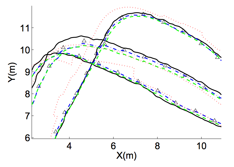
Here we see several paths from a robot moving in a rough loop from the paper’s test set. Ground truth $y_{0:t}$ is shown in black, $z_{0:t}$ shows as black triangles, RES is shown in blue dots and dashes, PRED in green dashes, and MEAS in red dots.

The obvious takeaway here is that the PRED method (green dashes) - optimizing your $Q$ and $R$ matrices for high confidence in the ground truth data - is optimal (among these approaches.) It only lags the others minimally on RMSE, but outperforms dramatically on log loss. Because the loss function formulation balances over confidence and under confidence, the filter tightly fits the ground truth data with an appropriate level of confidence.

JOINT and MEAS failed badly on log loss: they are so confident in their predictions that they assign low probability to the ground truth. Both setups seek high confidence on the current measurements, which are already incorporated in the EKF prediction in the first place. This extra emphasis on measurement confidence diminishes the value placed on the prior knowledge embedded in the motion model.

In the image above, MEAS is visibly prone to intermittent large corrections on new GPS readings. The authors also note that JOINT and MEAS are both vulnerable to correlated noise. By valuing the measurements too much, when the noise correlation drops, the measurement jumps, and the model’s state is out of position but holding a high confidence. Not good.

Conclusions

The major conclusions for me are:

1. You can learn optimal noise matrices, you don’t have to hand tune your noise matrices. This is a relatively simple procedure to set up, and well worth the time if you are working on a production system.
2. PRED is the best procedure, hands down, if you have ground truth data. Implementing that should get you pretty close to optimal performance for your motion model, measurement model, sensor suite and robot. And the implementation is straight forward and does not require substantial new calculations.
3. Model more of the system if possible, since that can reduce process noise. In robotics, where we have strong 3D motion models available, it’s good to go with the more complex models, all things being equal.
4. Be cautious if you don’t have ground truth. I was recently in this situation, and considered implementing something similar to MEAS. Given the results in Discriminant Training I would hesitate now. If I were to try it, I would do the following:
   • I might add regularization parameters to the MEAS loss function to discourage unreasonably low covariance and large jumps in model state.
   • Similarly, I would observe the model, looking for large jumps in position and overall self-consistency of the filter.
   • The motion model implemented in Discriminant Training included learning a bias term for the gyro. If I was going to optimize without ground truth, I would want to model a slow moving bias term in the GPS measurements.

I may, as time allows, try implementing this procedure.

What do you think? Have you run into problems like these before?

1. ResearchGate: How to find Q and R in Kalman Filter? ↩

2. ResearchGate: How do we determine noise covariance matrices Q & R? ↩

3. Discriminative Training of Kalman Filters, 2005, by Pieter Abbeel, Adam Coates, Michael Montemarlo, Andrew Ng, and Sebastian Thrun. ↩

4. How To NOT Make the Extended Kalman Filter Fail, 2013, by René Schneider and Christos Georgakis. ↩

Written on November 14, 2018